Hamiltonian paths tutorial

Introduction

Hamiltonian paths are rarely encountered in video games compared to "shortest path" algorithms like A*. This is partly because the Hamiltonian paths problem is notoriously difficult, but mostly because there haven't been enough open source projects, libraries or tutorials on the subject. This is a real shame since many genres of games could be designed around the use of Hamiltonian paths.

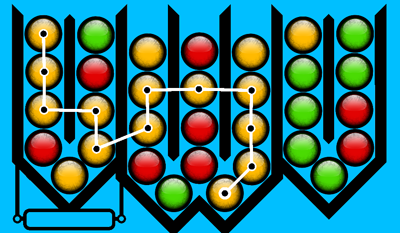
Diagram 1: Super Chains, a puzzle game developed by 2dengine.
Find the longest chain of bubbles sharing the same color.

Hamiltonian paths present a search problem that is considered "NP-hard". Some really sophisticated research has gone into this problem, so please consider this humble tutorial as a brief introduction.

Knight's tour problem

Imagine a regular 8x8 chessboard. Can you traverse every square on the board using only the knight piece? Here is the catch: you are only allowed to visit each square once! It takes exactly 63 moves to solve the puzzle and if you manage to do it, then you have found one possible "Hamiltonian path". Note that if you can finish the Knight's tour one move away from the initial square where you started then you have completed what is called a "Hamiltonian cycle".

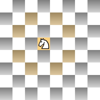
Diagram 2: Knight piece with eight possible moves highlighted in yellow.

Building the graph

Initially, it seems like Hamiltonian paths are an easy challenge for the computer. All we have to do is track the number of visited squares, right? Before we give it a try, let's refer to the chessboard as a "graph" and its squares as "vertices" or "nodes". Any possible move of the knight will be called an "edge". Why? Because technical nomenclature make us sound smart! When we draw all possible connections on the board then the terminology makes a little more sense:

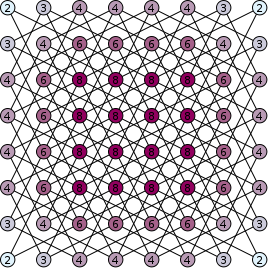
Diagram 3: Graph of the legal knight moves on a chessboard:
Lines are called "edges", where each edge connects two neighboring nodes
Circles are called "nodes" and each number represents the number of edges for that node

The graph is represented in Lua as a table where: 1.each key is a node and 2.each value is a table containing the neighboring nodes.
This simple approach allows us to check if any two nodes are connected by writing:

if graph[node1][node2] then -- node1 and node2 are connected

Next, we are going to build a graph representing the chessboard. Each node or square on the board will be labeled with a number (from 1 to 64 for an 8x8 board). To connect the nodes, we need a way to find all the legal knight moves for any given square. The following example uses a method called "mailboxing". Mailboxing adds a few rows of padding and allows us to eliminate invalid moves, so that our poor knight can't jump off the board! If you have any chess knowledge at all, you could probably come up with a different approach of generating the graph.

-- mailbox
local w, h = 8, 8
local squares = {}
local sq = 1
for y = 3, h + 2 do
  local i = (y - 1)*(w + 2)
  for x = 2, w + 1 do
    squares[i + x] = sq
    sq = sq + 1
  end
end

-- graph
local knight = { -21, -19, -12, -8, 8, 12, 19, 21 }
local graph = {}
for from, sq in pairs(squares) do
  graph[sq] = {}
  for _, move in pairs(knight) do
    local to = from + move
    local sq2 = squares[to]
    if sq2 then
      graph[sq][sq2] = true
    end
  end
end

Traversing the graph

We know for a fact that the Knight's tour problem can be solved with 63 moves. If we include the starting square that's a path of 64 squares.
Generally, we can figure out the longest, theoretically possible Hamiltonian path for any graph using the formula:

maxdepth = numberOfNodes - max(nodesWithOnlyOneEdge - 2, 0)

This value is important, because it serves as an upper bound while searching for a solution.
To estimate the length of the longest Hamiltonian path, we use the following code:

-- count the number of edges for a node
function count(edges)
  local n = 0
  for neighbor in pairs(edges) do
    n = n + 1
  end
  return n
end

-- estimate the longest Hamiltonian path
function maxdepth(graph)
  local n = 0
  local edge1 = 0
  for node, edges in pairs(graph) do
    if count(edges) == 1 then
      edge1 = edge1 + 1
    end
    n = n + 1
  end
  return n - math.max(edge1 - 2, 0)
end

Brute force

OK, though guy... you recently upgraded your CPU and think you can plow through the Hamiltonian path problem in no time. The bad news is that that there are estimated 4x10⁵¹ possible move sequences and the valid solutions are quite rare. Now that you have an idea of the enormous size of the search space, it should be clear that using "brute force" is clearly not an option.

Warnsdorf's rule

While there are linear-time algorithms for solving the Knight's tour, this is not the case for more complicated types of graphs. Nevertheless, mathematicians have discovered a few clever tricks. Warnsdorf's rule suggest that when searching the graph, we should seek the nodes that have the fewest non-visited neighbors. Let's look at a concrete example.

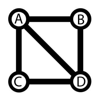
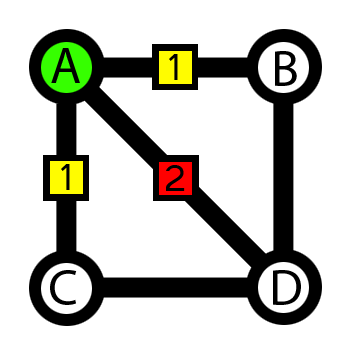
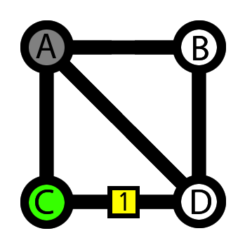
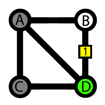
Diagram 4: Graph traversal following Warnsdorf's rule
1. Graph of four nodes (A,B,C and D) and five edges, traversal begins from node A.
2. Node A: There are three possible choices (B,C and D). Two of the choices (B and C) have fewer non-visited neighbors compared to the third choice (D). According to Warnsdorf, choices B and C must be considered before D.
3. Node C: There is one possible choice (D)
4. Node D: There is one possible choice (B)

Warnsdorf's rule is good for simple graphs like our chessboard, but it may not always work. In many cases, following the rule is not enough to find a solution. Therefore, our code needs to perform some backtracking.

local visited = {}

-- count the number of non-visited neighbors
function nonvisited(edges)
  local n = 0
  for neighbor in pairs(edges) do
    if not visited[neighbor] then
      n = n + 1
    end
  end
  return n
end

-- traverse the graph using Warnsdorf's rule
function traverse(graph, node, depth, best, path)
  depth = depth or maxdepth(graph)
  path = path or {}
  best = best or {}
  -- track the longest path
  table.insert(path, node)
  if #path > #best then
    for i = 1, #path do
      best[i] = path[i]
    end
  end
  -- visit neighboring nodes
  if #best < depth then
    visited[node] = true
    -- consider all non-visited neighbors
    local choices = {}
    for neighbor in pairs(graph[node]) do
      if not visited[neighbor] then
        table.insert(choices, neighbor)
      end
    end
    -- sort choices by fewest non-visited neighbors
    table.sort(choices, function(a, b)
      return nonvisited(graph[a]) < nonvisited(graph[b])
    end)
    -- try each available choice
    for i = 1, #choices do
      if traverse(graph, choices[i], depth, best, path) then
        break
      end
    end
    visited[node] = nil
  end
  table.remove(path)
  return #best == depth, best
end

Choosing a starting node

Note that with the Knight's tour problem we can start the search from any square, but for other types of graphs some starting nodes could be eliminated.
For the purposes of this tutorial, we want to keep it simple. Using the "traverse" algorithm is as easy as providing a graph and a starting node:

-- search for Hamiltonian paths
local res, path = traverse(graph, 1)
-- print the longest path found
error("found path:" .. table.concat(path,','))

I would like to end this tutorial by saying that the code provided here is far from perfect. The methods we have considered are just slightly more advanced than using brute force, but the difference in speed is significant. The tutorial code could probably handle most small graphs in less than a second, but imagine what may be possible with more sophisticated techniques! More importantly, I hope to have encouraged you to learn about graph theory. Thanks for reading and have a nice day.

References

Knight's Tour on Wikipedia